One of the principles of economic theory is that price will adjust so that supply and demand match. This way of thinking about allocation actually turns out to be very useful even for situations where price adjustment is not used as a market clearing mechanism. To understand this, we start with a pure supply and demand example.

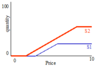
Suppose that there are two suppliers with the supply curves shown below:

and that there are two demanders with the demand curves shown below:

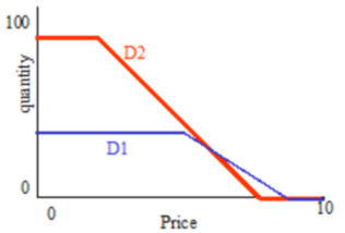
We can find a market equilibrium by adding up the two supply curves to form a market supply curve, adding up the two demand curves to form a market demand curve, and then finding the point where the two curves intersect:

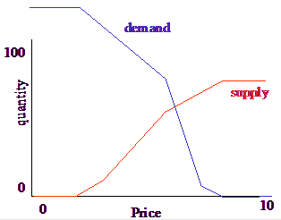
Once we find that price, about 7, we just go back to the original supply and demand curves to determine how much each supplier supplies, and how much each demander demands.

Now consider the case where there is some fixed market demand and we want to determine how it is divided between the two suppliers. Thus we treat the market demand as constant, and determine the price where it intersects the supply curves.

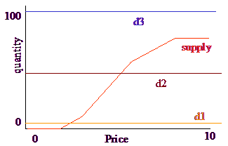
If the demand is small, such as at d1, only supplier s2 supplies anything. At demand d2 both suppliers supply something. If the demand is d3, supply never meets demand so we can’t determine price. It is clear, however, that both suppliers should supply all they can.

In the earlier section we were talking about priority, and now we are talking about price. While the two seem related, they are not the same thing. In fact as the example was posed the decision about what to buy was a decision by demanders based on preference not a decision by suppliers based on price. However, all we need to do is flip the supply curve and change the label on the x axis to get that interpretation:

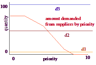
If demand is low (d1), the highest priority suppliers are used. When demand is higher (d2), more suppliers are used. If the demand is very high (d3) then all suppliers are used to their capacities.

What we have created then, is a graphical way of solving the one-to-many or many-to-many allocation problem. We can interpret this as either a market based balancing of supply and demand, or a rationing scheme based on the preferences of the agent being rationed to. The underlying curves can be made to respect the capacities of the agents, and the preferences of agents can me represented by selecting different shapes and positions.

This approach is a generalization of the approach and algorithm developed by William T. Wood in the 1980s to solve the one-to-many allocation problem using prioritization curves such as the ones illustrated above.

The curves used to represent prioritizations need to be nonnegative, continuous and monotone. More specifically, demand curves need to slope down and supply curves need to slope up. In addition, there are two restrictions on shape that, though they are not strictly necessary for this approach to allocation to work, do make sense.

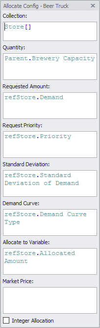
•There should some price or priority beyond which the quantity will no longer increase. This might be due to hard constraints on capacity for supply, or satiation for demand.

•There should be some price or priority beyond which the quantity gets very small or actually becomes 0.

Generally this leads to curves that are roughly S shaped and characterized by their midpoint, and the distance over which they are spread. In Ventity, curves are specified by the midpoint (Priority) and the spread (Standard Deviation). The specific curve shape is the integral of a Gaussian (Normal) curve.

In addition to this shape, Ventity supports a truncated constant elasticity curve. The equation for constant elasticity is

quantity = A(priceε),

where the elasticity ε is positive for supply curves and negative for demand curves. For demand curves as price goes toward 0, the quantity becomes infinite and this is why the constant elasticity demand curves are truncated (satiation) at a minimum price and the supply curves are truncated (capacity) at a maximum price. In most cases these truncations will not matter as the price will be within the normal range of behavior.

Letting qo be the quantity passed we would have, for a demand curve:

q(x) = q0 * (x/ppriority)^(-pextra) if x > pwidth

q(x) = q0 * (pwidth/ppriority)^(-pextra)if x <= pwidth

Whereas for a supply curve we would have (see below for more discussion on supply/demand):

q(x) = q0 * (x/ppriority)^(pextra) if x < pwidth

q(x) = q0 * (pwidth/ppriority)^(pextra)if x >= pwidth

Supply curves slope up, while demand curves slope down. Ventity determines which type of curve it is from the input field.

Collection: The collection of entities to which your resource will be allocated.

Quantity: The fixed total to be divided among entities in the collection

Requested Amount: The maximum amount desired (or offered) by each entity in the collection. This is specified using the special reference refEntityType, where EntityType is the entity type in the collection. For example, in the illustration to the left, refStore.Demand tells Ventity to use the value of variable "Demand" for each Store entity in the collection.

Reference Priority: The priority that each entity in the collection will receive in the allocation. If an entity has higher values than other entities, that entity will get more of its demand met in conditions of scarcity.

Standard Deviation: The "width" of the demand curve.

Demand Curve: Currently inoperative, this field will be used to choose which family of demand curve is being used.

Allocate to Variable: The variable in each entity in the collection whose value will be set to the amount received in the allocation. Two important notes:

1. This variable must be in refEntityType, where EntityType is the type of entity in the collection (see above).

2. The expression for this variable, where it is defined, must be equal to the allocation function Allocation().

Market Price: currently inoperative.

Integer Allocation: When checked, allocations are made in whole numbers.

Market Actions are similar, but the same options are presented both for a collection of suppliers and for a collection of demanders. The variable listed in "Allocate to Variable" is set to the amount supplied or demanded by each entity in each collection. As with Allocate actions, these "Allocate to" variables must be set equal to to the special function Allocation(), with no arguments.